


COMPOSITION
-
Photography basics: Camera Aspect Ratio, Sensor Size and Depth of Field – resolutions
Read more: Photography basics: Camera Aspect Ratio, Sensor Size and Depth of Field – resolutionshttp://www.shutterangle.com/2012/cinematic-look-aspect-ratio-sensor-size-depth-of-field/
http://www.shutterangle.com/2012/film-video-aspect-ratio-artistic-choice/


-
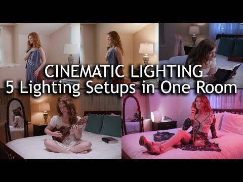
9 Best Hacks to Make a Cinematic Video with Any Camera
Read more: 9 Best Hacks to Make a Cinematic Video with Any Camerahttps://www.flexclip.com/learn/cinematic-video.html
- Frame Your Shots to Create Depth
- Create Shallow Depth of Field
- Avoid Shaky Footage and Use Flexible Camera Movements
- Properly Use Slow Motion
- Use Cinematic Lighting Techniques
- Apply Color Grading
- Use Cinematic Music and SFX
- Add Cinematic Fonts and Text Effects
- Create the Cinematic Bar at the Top and the Bottom


DESIGN
-
Pantheon of the War – The colossal war painting
Read more: Pantheon of the War – The colossal war paintingFour years in the making with the help of 150 artists, in commemoration of WW1.
edition.cnn.com/style/article/pantheon-de-la-guerre-wwi-painting/index.html
A panoramic canvas measuring 402 feet (122 meters) around and 45 feet (13.7 meters) high. It contained over 5,000 life-size portraits of war heroes, royalty and government officials from the Allies of World War I.
Partial section upload:


COLOR
-
About color: What is a LUT
Read more: About color: What is a LUThttp://www.lightillusion.com/luts.html
https://www.shutterstock.com/blog/how-use-luts-color-grading
A LUT (Lookup Table) is essentially the modifier between two images, the original image and the displayed image, based on a mathematical formula. Basically conversion matrices of different complexities. There are different types of LUTS – viewing, transform, calibration, 1D and 3D.


-
Gamma correction
Read more: Gamma correction

http://www.normankoren.com/makingfineprints1A.html#Gammabox
https://en.wikipedia.org/wiki/Gamma_correction
http://www.photoscientia.co.uk/Gamma.htm
https://www.w3.org/Graphics/Color/sRGB.html
http://www.eizoglobal.com/library/basics/lcd_display_gamma/index.html
https://forum.reallusion.com/PrintTopic308094.aspx
Basically, gamma is the relationship between the brightness of a pixel as it appears on the screen, and the numerical value of that pixel. Generally Gamma is just about defining relationships.
Three main types:
– Image Gamma encoded in images
– Display Gammas encoded in hardware and/or viewing time
– System or Viewing Gamma which is the net effect of all gammas when you look back at a final image. In theory this should flatten back to 1.0 gamma.
(more…) -
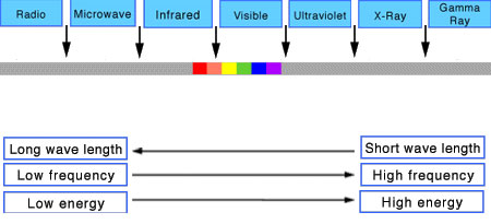
Photography basics: Lumens vs Candelas (candle) vs Lux vs FootCandle vs Watts vs Irradiance vs Illuminance
Read more: Photography basics: Lumens vs Candelas (candle) vs Lux vs FootCandle vs Watts vs Irradiance vs Illuminancehttps://www.translatorscafe.com/unit-converter/en-US/illumination/1-11/

The power output of a light source is measured using the unit of watts W. This is a direct measure to calculate how much power the light is going to drain from your socket and it is not relatable to the light brightness itself.
The amount of energy emitted from it per second. That energy comes out in a form of photons which we can crudely represent with rays of light coming out of the source. The higher the power the more rays emitted from the source in a unit of time.
Not all energy emitted is visible to the human eye, so we often rely on photometric measurements, which takes in account the sensitivity of human eye to different wavelenghts


Details in the post
(more…)


LIGHTING
-
ICLight – Krea and ComfyUI light editing
Read more: ICLight – Krea and ComfyUI light editing
https://drive.google.com/drive/folders/16Aq1mqZKP-h8vApaN4FX5at3acidqPUv
https://github.com/lllyasviel/IC-Light
https://generativematte.blogspot.com/2025/03/comfyui-ic-light-relighting-exploration.html

Workflow Local copy

-
Simulon – a Hollywood production studio app in the hands of an independent creator with access to consumer hardware, LDRi to HDRi through ML
Read more: Simulon – a Hollywood production studio app in the hands of an independent creator with access to consumer hardware, LDRi to HDRi through MLDivesh Naidoo: The video below was made with a live in-camera preview and auto-exposure matching, no camera solve, no HDRI capture and no manual compositing setup. Using the new Simulon phone app.
LDR to HDR through ML
https://simulon.typeform.com/betatest
(more…)Process example
-
Disney’s Moana Island Scene – Free data set
Read more: Disney’s Moana Island Scene – Free data sethttps://www.disneyanimation.com/resources/moana-island-scene/
This data set contains everything necessary to render a version of the Motunui island featured in the 2016 film Moana.

-
9 Best Hacks to Make a Cinematic Video with Any Camera
Read more: 9 Best Hacks to Make a Cinematic Video with Any Camerahttps://www.flexclip.com/learn/cinematic-video.html
- Frame Your Shots to Create Depth
- Create Shallow Depth of Field
- Avoid Shaky Footage and Use Flexible Camera Movements
- Properly Use Slow Motion
- Use Cinematic Lighting Techniques
- Apply Color Grading
- Use Cinematic Music and SFX
- Add Cinematic Fonts and Text Effects
- Create the Cinematic Bar at the Top and the Bottom
-
Christopher Butler – Understanding the Eye-Mind Connection – Vision is a mental process
Read more: Christopher Butler – Understanding the Eye-Mind Connection – Vision is a mental processhttps://www.chrbutler.com/understanding-the-eye-mind-connection
The intricate relationship between the eyes and the brain, often termed the eye-mind connection, reveals that vision is predominantly a cognitive process. This understanding has profound implications for fields such as design, where capturing and maintaining attention is paramount. This essay delves into the nuances of visual perception, the brain’s role in interpreting visual data, and how this knowledge can be applied to effective design strategies.
This cognitive aspect of vision is evident in phenomena such as optical illusions, where the brain interprets visual information in a way that contradicts physical reality. These illusions underscore that what we “see” is not merely a direct recording of the external world but a constructed experience shaped by cognitive processes.
Understanding the cognitive nature of vision is crucial for effective design. Designers must consider how the brain processes visual information to create compelling and engaging visuals. This involves several key principles:
- Attention and Engagement
- Visual Hierarchy
- Cognitive Load Management
- Context and Meaning


COLLECTIONS
| Featured AI
| Design And Composition
| Explore posts
POPULAR SEARCHES
unreal | pipeline | virtual production | free | learn | photoshop | 360 | macro | google | nvidia | resolution | open source | hdri | real-time | photography basics | nuke
FEATURED POSTS
-
What Is The Resolution and view coverage Of The human Eye. And what distance is TV at best?
-
Top 3D Printing Website Resources
-
Eyeline Labs VChain – Chain-of-Visual-Thought for Reasoning in Video Generation for better AI physics
-
Sensitivity of human eye
-
Photography basics: How Exposure Stops (Aperture, Shutter Speed, and ISO) Affect Your Photos – cheat sheet cards
-
Photography basics: Exposure Value vs Photographic Exposure vs Il/Luminance vs Pixel luminance measurements
-
Guide to Prompt Engineering
-
Gamma correction
Social Links
DISCLAIMER – Links and images on this website may be protected by the respective owners’ copyright. All data submitted by users through this site shall be treated as freely available to share.
